
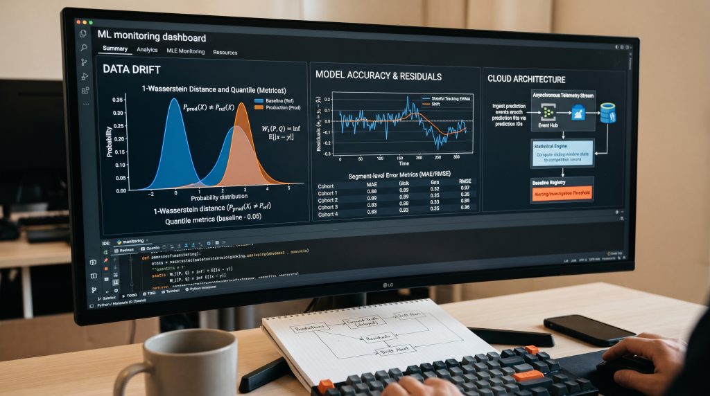
As we’ve moved from static analytical models to deploying advanced machine learning (ML) systems in production, we’ve solved the challenge of capturing complex, nonlinear relationships in our data. However, deploying a model is only the beginning of its lifecycle. The real world is dynamic, and a model that performs exceptionally well during offline evaluation can degrade as the environment changes.
This post presents our practical, cloud-native approach to monitoring ML models in production. We focus on the architecture and mathematical frameworks required to build a robust cloud service that continuously compares real-time data and model performance against historical dataset statistics, quantiles, and baseline performance.
The Silent Failures: Data Drift vs. Model Drift
Before architecting a monitoring service, it is critical to define what exactly we are looking for. Production ML systems can degrade for several different reasons, two of the most important being changes in the input distribution and changes in the relationship between inputs and outcomes.
1. Data Drift
Data drift occurs when the distribution of one or more model inputs changes over time:
Pprod(X) ≠ Pref(X)
Covariate shift is the specific case where the input distribution changes while the conditional relationship between inputs and the target remains approximately constant:
Pprod(Y|X) ≈ Pref(Y|X)
For example, if a sensor begins degrading and systematically produces lower values, the production feature distribution may move away from the distribution observed in the reference dataset. This is an important signal, although it does not necessarily mean that model performance has already degraded.
2. Concept Drift
Concept drift occurs when the relationship between the inputs and the target changes:
Pprod(Y|X) ≠ Pref(Y|X)
Concept drift can occur even when the input distributions appear stable. For example, customer behavior may change while the distribution of customer attributes remains largely unchanged.
These distinctions matter operationally. Data drift can often be detected immediately because features are available at prediction time. Concept drift is generally harder to detect because it requires observations of the actual outcome, which may only become available after a significant delay.
Architecting the Cloud Monitoring Service
To catch these changes before they impact downstream operations, we maintain an independent, always-on cloud monitoring service. Rather than tightly coupling monitoring to the inference server, we use an asynchronous, event-driven architecture, often built on managed services such as AWS Kinesis, GCP Pub/Sub, or Azure Event Hubs.
The architecture consists of three main components:
1. The Telemetry Stream
Every time the ML model makes a prediction, the inference service emits a prediction event containing a unique prediction ID, model ID and version, timestamp, feature-schema version, input features or feature references, and prediction ŷt.
These events are published to an event stream and persisted in a durable data store for later analysis.
When the actual ground truth becomes available — which may be delayed by hours, days, or longer — the label event is associated with the original prediction using the prediction ID. This is preferable to relying solely on timestamps, particularly when predictions and labels can arrive out of order.
The explicit model version is also important when multiple model versions are deployed simultaneously. Monitoring data must be associated with the model version that generated the prediction so that performance and drift are never accidentally compared against the baseline of a different model.
2. The Statistical Engine
A scheduled cloud function, streaming job, or distributed processing job computes sliding-window statistics over production data.
Depending on the feature type, the statistical engine can calculate quantiles, distribution distances, missing-value rates, categorical-frequency changes, and other data-quality and drift metrics.
3. The Baseline Registry
A versioned storage layer contains the statistical profiles generated from a defined reference dataset, such as the training, validation, or representative pre-production population.
The baseline registry should be associated with the relevant model version, feature schema, reference dataset version, and monitoring configuration. This ensures that production observations are compared against the correct reference rather than against an unrelated model or dataset.
Monitoring Data Drift via Quantiles and Distributions
Because ground truth is often delayed, data drift is one of the first signals available after deployment. Our monitoring service continuously compares production feature distributions against those of the reference dataset.
Instead of relying only on the mean and variance, our service tracks the distribution of each important feature using quantiles. Let Qq(Xref) denote the q-th quantile of a feature in the reference dataset, and Qq(XW) the corresponding quantile in the production window W.
Quantiles provide a compact representation of the distribution and make it possible to detect changes in its center and tails. For example, comparing the 50th, 90th, 95th, and 99th percentiles can reveal a change that would be hidden by monitoring only the mean and standard deviation.
For continuous one-dimensional variables, these quantiles can also be used to estimate the 1-Wasserstein distance. The distance can be expressed in terms of the inverse cumulative distribution functions:
W1(P, Q) = ∫01 |FP−1(u) − FQ−1(u)| du
where F−1 denotes the quantile function.
In a production implementation, the integral can be approximated over a grid of quantile levels:
Ŵ1 ≈ ∑i |Qprod(qi) − Qref(qi)| Δq
This allows the monitoring service to use a quantile-based representation while still producing a single distribution-distance statistic for alerting.
For categorical variables, other measures such as population stability index (PSI), Jensen-Shannon divergence, or changes in category frequencies may be more appropriate.
Calibrating Drift Thresholds
To quantify the divergence between the production distribution P and the reference distribution Q, we employ the Wasserstein Distance, also known as Earth Mover’s Distance. For continuous variables, the 1-Wasserstein distance is defined as:
W1(P, Q) = infγ ∈ Π(P, Q) 𝔼(x, y) ~ γ [|x − y|]
where Π(P, Q) is the set of joint distributions γ whose marginals are P and Q.
The monitoring service computes this statistic over a defined sliding window and compares it against a threshold calibrated from historically stable production or validation periods.
Rather than relying on a universal threshold such as 3σ, the threshold should account for factors such as window size, feature variability, seasonality, and the desired false-positive rate.
In practice, an empirically determined percentile of the drift statistic observed during known-stable periods can provide a more robust alerting threshold. For example, the service might alert when the observed Wasserstein distance exceeds the 99th percentile of distances historically observed between comparable stable windows.
Thresholds can also be configured separately for individual features based on their operational importance and expected variability.
Tracking Real-Time Model Accuracy
When ground truth data arrives, the service shifts from monitoring feature distributions to evaluating actual model performance.
Just as we did during training, we track standard metrics such as Mean Absolute Error (MAE) and Root Mean Squared Error (RMSE). However, computing a single global error metric is insufficient for production.
Instead, we monitor the distribution of residuals over time:
et = yt − ŷt
Under stable conditions, the residual distribution should remain broadly consistent with the reference behavior. This includes not only its mean but also its scale and tails.
The cloud service therefore maintains stateful tracking of residuals using an Exponentially Weighted Moving Average (EWMA), which gives more weight to recent observations:
Zt = λet + (1 − λ)Zt−1
where 0 < λ ≤ 1 controls how quickly the statistic responds to recent changes.
A persistent shift in the EWMA away from its reference level is a useful signal of systematic prediction bias or performance degradation. However, a residual shift alone does not prove that concept drift has occurred.
Changes in upstream data pipelines, label-generation processes, sensor calibration, or other operational conditions can also affect residuals.
For this reason, the monitoring service combines residual-based signals with feature-distribution monitoring, target-distribution monitoring where labels are available, and segment-level performance metrics. A sustained change across several independent signals provides stronger evidence that the underlying relationship between inputs and outcomes may have changed.
The same principle applies to residual variance. A model can maintain an approximately zero residual mean while its error variance increases substantially. Monitoring both location and scale therefore provides a more complete picture of model performance.
Monitoring Performance Across Data Segments
Computing an overall MAE or RMSE can hide localized failures.
We therefore slice performance metrics across predefined segments, such as prediction-value quantiles, important feature ranges, geographic regions, customer segments, or other operational cohorts.
For example, a model may maintain an acceptable overall MAE while its performance in the upper 5% of predicted values deteriorates significantly.
By comparing real-time performance across these segments against the corresponding reference benchmarks, the monitoring service can identify failures that would otherwise be hidden by aggregate metrics.
This is particularly important when the business impact of errors is not uniform across the input space.
Next Step: Automated Remediation
Building a cloud service that alerts you to data and model drift is a major step forward in MLOps maturity. The next phase of our infrastructure evolution focuses on automated remediation.
When the statistical engine detects sustained drift or a significant performance degradation, it can trigger a controlled investigation or a shadow retraining pipeline using recent production data.
However, not every drift event requires retraining. A temporary seasonal change, an upstream data-quality issue, or a legitimate change in the operating environment may produce a drift signal without requiring a new model.
Automated retraining should therefore remain subject to validation and deployment controls. The candidate model should be evaluated against appropriate holdout data and production-like scenarios before it replaces the currently deployed model.
By treating models as living systems and maintaining a dedicated monitoring service, we can detect changes in their statistical and predictive behavior early. The monitoring layer creates a controlled feedback loop between production observations and model operations: detect drift, investigate the underlying cause, evaluate whether model performance has actually degraded, and only then trigger retraining or other remediation.
The goal is not to guarantee that a model will remain unchanged in a changing environment. It is to make changes observable, measurable, and actionable so that production ML systems can evolve safely as the real world evolves.